Getting Up and Running with Essbase Part 3

Now that Essbase is more or less up and running, what else is there to do on a twelve-hour flight except put a couple of Essbase cubes together, to see how the process works and compare it to Analytic Workspace Manager? As a quick recap, I’ve got Essbase (a.k.a. Hyperion Analytic Services) 9.3.1 installed, along with Hyperion Analytic Integration Services, Hyperion Analytic Services Client, Hyperion Shared Services and the license server, and they’re all configured and up and running except Shared Services, which seems to be working ok although the configuration utility says that it needs reconfiguration. So, where do we start?

Although you can build Essbase cubes manually, as you can with Oracle OLAP (through OLAP DML or PL/SQL) and Express (Express SPL), there’s a tool called Hyperion Essbase Integration Services that does a similar job to Analytic Workspace Manager (AWM); you can define the dimensional model, add calculated measures and aggregation plans, map the cube to relational data sources and then load the cube and aggregate it. Integration Services is a little bit different to AWM in that it actually has a repository and runs as a mid-tier service, but the principle is pretty much the same.

Going back to posting I put together earlier today on Essbase concepts, an Essbase cube consists of the usual dimensions, measures, hierarchies and so forth, but you also get a database outline as well, which is a container for all the dimensional metadata that in Oracle OLAP is sort of stored in the OLAP Catalog, but also in the analytic workspace data dictionary.

When you start to work with Integration Services, you get to build these dimensional objects and the outline by deriving the cube metadata from a relational star or snowflake schema, and so as a good place to start off I thought I’d try and build a cube using the Global Electronics sample dataset that you can download from OTN, which is also of course interesting because it’s the standard demo dataset for Oracle OLAP.

With Integration Services, building a cube is a four-step process (pic courtesy of the Essbase Integration Services Data Preparation Guide)

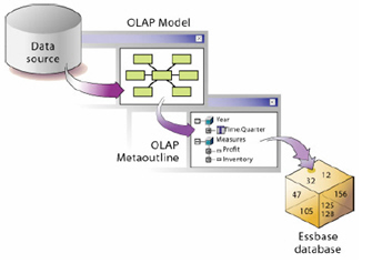
The first step is to locate your relational data source, which really should be a star or snowflake schema – if it’s not, the recommendation is that you stage it to get it into a denormalized, star schema format. Make sure it’s got foreign key links between the fact and dimension tables, and then either create an ODBC or Oracle Net connection to the schema or database. Also, a quick note on the Global schema – I had to remove the double quotes (“) from entries in the PRODUCT_DIM.ITEM_DSC column to get the cube to load properly, you’ll need to do this as well if you’re going to follow along with the example.

Starting up Integration Services, I select New from the application menu to display the Welcome dialog.

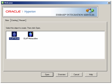
As the first step in building an Essbase cube using Integration Services is to build an OLAP Model, I select this option and press Open to start creating a new OLAP Model.

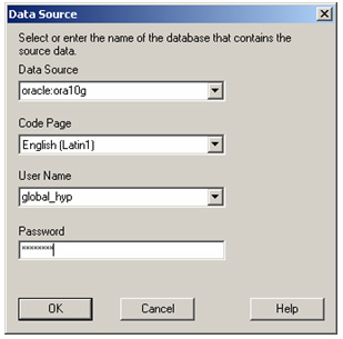
The first thing that’s displayed is a dialog asking me for details of a data source. Using this dialog, I can either enter the details of an ODBC connection, or an Oracle connection string if I use the prefix “oracle:”. I’ve copied the Global Electronics tables into a separate schema called GLOBAL_HYP, so I put in the details for this schema and press OK to connect to the database and open the Integration Services Console.

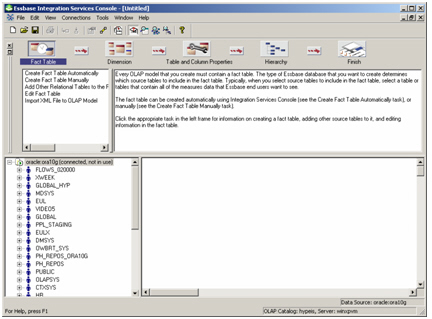
The Integration Services Console has three sections to it:

1. A “help” section at the top that guides you through the steps in creating a model
2. A list of schemas down the left-hand side, where each schema expands out to the tables and views that you can drag on to the right-hand side
3. An area on the right-hand side where you lay out the star schema you’ve chosen.

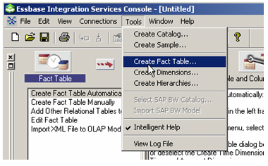
There are various ways I can build up the star schema using this tool, including following the help steps, dragging and dropping tables from the schema diagram on the left, or in my case, selecting Tools > Create Fact Table from the application menu.

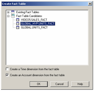
I then select the UNITS_FACT table from the global schema, uncheck the time dimension checkbox (I’ll create this manually in a second) but leave the account dimension checkbox ticked – account dimensions are “dimensions of measures” that Essbase sets up, I might as well get the tool to create this as it’s just a case of create it and leave it, you don’t do much with it afterwards (at least I don’t think you do).

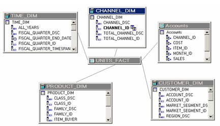
I then repeat the process for the dimensions, selecting Tools > Create Dimension, add them to the diagram, and end up with something like this (note that the Account dimension created earlier is actually a dimension of measures, we’ll lose the dimension keys later on).

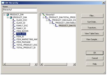
Now I need to create at least one hierarchy per dimension. I do this by double-clicking on each dimension, selecting the Hierarchy tab from the dimension properties dialog, and then selecting the dimension members in much the same way as AWM or Discoverer Administrator.

When it comes to the Time dimension, I set the dimension type to Time using the dimension properties dialog, and then create the hierarchy as normal. There’s no end date, timespan or any other time-specific attributes to set here, I suspect there is some more work to do on this though but I just haven’t spotted it yet.

Now all the model details are specified, I can save the model and move on to creating the Metaoutline. To do this, I select File > Close from the application menu, and then File > New to go back to the Welcome screen, then press the Metaoutline button and base it on the model I’ve just created.

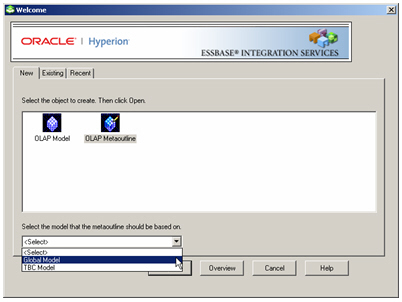
I’m prompted again to put the password in for the global schema, and then the Integration Services Console opens up again, but this time to edit the Metaoutline.

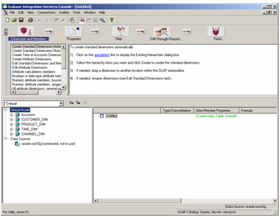
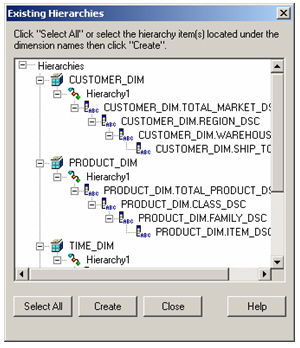
If you’ve got the Intelligent Help section option, as I have in the screenshot above, creating the metaoutline is pretty straightforward and just involves making sure the Dimensions and Members button is selected, and then clicking on the Autodetect link in the help text. Integration Services Console will then look at the dimensional and hierarchical structure in your model, and create the dimensional part of the metaoutline for you.

Then it’s just a case of dragging the Accounts dimension across as well, and then the measures in the fact table/accounts dimension that you want to include in the cube, and that’s the metaoutline created.

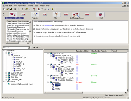
Notice how it’s marked the Time dimension as dense, and the rest as sparse, just like AWM normally does – I can change this if I want to, along with the aggregation method for each measure, by right-clicking on each item and using the properties dialog, but I leave this for now and go with the defaults.

Before I can start loading up the cube though, there’s one more thing to do – actually create the OLAP database to put the cube in to. To do this, I start up Analytic Administration Services, log in as “admin”/”password” and navigate to the section where my Analytic Server (Essbase server) is located. I then right-click on it and select Create Application > Using Block Storage.

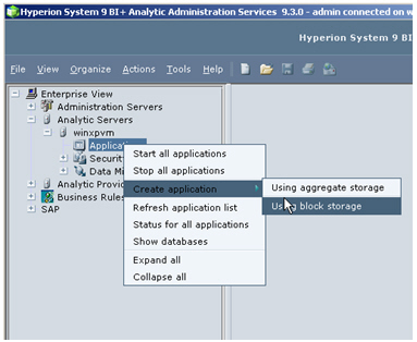
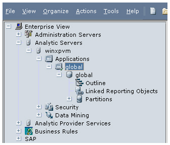
I call the application “Global” and then create a database under it, also called Global. Now I’m ready to load up some data.

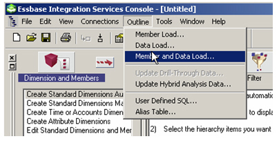
Going back to Integration Services Console, I select Outline > Member and Data Load to start the load process.

The console now shows a dialog that allows me to select the application and database to load data in to, and to select the calculation script to use – this bit is important, if you leave it at the default, your measures won’t get aggregated and all you’ll get is lots of missing values when you try and view the cube.

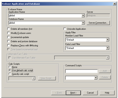
Then, after pressing Next, I’m asked whether I want to run the load now or later on, I choose now and let the load process start. A progress screen then shows me the status of the load, in a similar way to AWM when you load a cube.

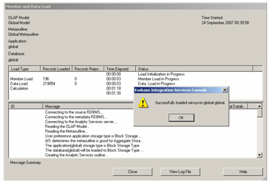
Once it’s all loaded and aggregated OK, you can switch back to the Analytic Administration Services tool and use the database preview feature to take a look at the data.

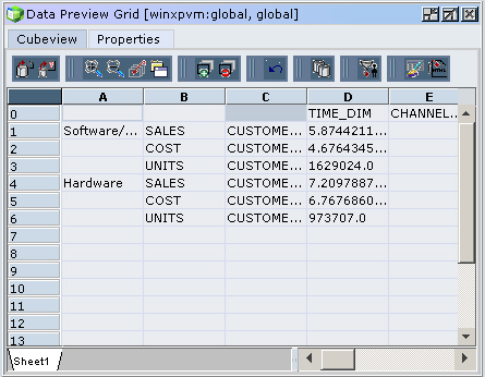
So there we go, a fairly basic cube created using Analytic Administration Services, Analytic Integration Services and the Global sample schema. I obviously haven’t looked at parent-child, ragged hierarchies and so forth, or started to take a look at the other storage type, Aggregate Storage Option, but it’s encouraging to at least get a cube up and see how the process works. That’s it for a bit now, but hopefully later on next week I’ll get a chance to look at the various OLAP front-ends that come packaged with Hyperion BI+, and maybe even try and turn my hand to a bit of MDX…