Oracle BI EE 10.1.3.4.1 – Single Table Repository Design – Modeling Statistics of common Sports – Tennis, Football etc – Part 2
In the last blog entry i had shown a simple scenario of creating a BMM layer for one physical table. In today’s entry i will be covering a practical use case of creating a BMM layer from one physical table. This is a very interesting use case and can be used to demonstrate the reporting capabilities of BI EE.
Any parent body of a sporting event involving 2 teams/individuals like Tennis/Football etc generally collects a plethora of statistics. In fact stats are more important in a sporting event directly (for placing bets, buying a team, Potential Sponsors, Player analyzing weakness of opponent etc) than any BI implementation for a business(direct impact is more obvious in sports). The stats from a sporting event has immediate impact and actually makes more sense for any person since the end user looking at the stats has more understanding of the game (i always feel that we can relate more to a sporting event than the functioning of a business, but that’s just me :-)).
Stats for any game involving 2 teams/individuals are collected at the game level. For example, if you consider tennis, the stats like number of shots, number of unforced errors , number of forced errors, Winning Points, Losing Points, set scores etc made by both the individuals are recorded as attributes to the game in a single row. For example, if you consider the screenshot below
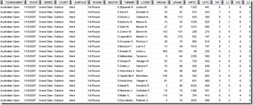
this contains actual data of all the games from 2007 in Men’s ATP tennis (i had to choose tennis since i thought that’s the game everyone can relate to). If you notice, every row corresponds to a game played by the winner & loser of the game. Typical stats are analyzed at a player level. For example, a major shoe manufacturer, before sponsoring a tennis player, would like to know the number of games won & lost by the player in the most commonly played surface (hard courts) for example. But if you look at the way the data is maintained, the KPIs for 2 players are maintained in the same row (winner as well as the loser). Writing reports even in plain SQL can be tricky since either the query has to involve multiple Unions or sub-query joins. All we have is a single table but with a rich set of stats that can be analyzed in multiple ways. The even more trickier part is in modeling this for reporting in BI EE.
For modeling this, we need to determine how any person would be analyzing the stats. As with any game, we always have our favorite players and not so favorite ones. And typically we want to analyze how each one of them performed against each other over a period of time. Also there are stats that we need to look at by not comparing with any other individual like number of matches played in a year, win percentage, loss percentage etc. So there are 3 kinds of stats
- Metrics when your favorite player is the winner – Example: Number of Matches Won
- Metrics when your favorite player is the loser – Example: Number of Matches Lost
- Metrics when your favorite player is the winner as well as the loser – Example: Number of Matches Played
As a first step we start with determining the logical tables that we will be needing in our model. They are
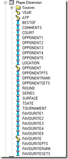
- Player Dimension – This logical table will contain the following attributes(screenshot). The winner & loser have been transformed to Favorite & Opponent. They do not map 1:1 though. We will be seeing how we map the Favorite & Opponents from Winner & Loser attributes later.
 2. Winner Facts
3. Loser Facts
4. All Facts

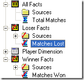
So, the idea is we enable a capability for any user to analyze the stats (Matches Won, Lost & Played) for their favorite players. But if you remember our data had 2 set of KPIs in a single row. That is our favorite player can be a winner as well as a loser. To accommodate this we create a couple of aliases in the Physical layer. One for Wins and the other for Losses.

There will not be any physical layer joins across these tables/aliases. The aliases that we have created above will act as 2 separate tables providing the 2 sets of KPIs in a single row. Since our perspective of analysis is FAVORITE & OPPONENT, we need to ensure that both the Winner as well as the loser are mapped to both FAVORITE & OPPONENT. So, we start with mapping the dimension to both the aliases. ATP-Winner alias will map Winner to Favorite & Loser to Opponent.

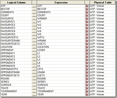
ATP-Loser alias will map Loser to Favorite & Winner to Opponent. Also the other attribute stats like Set Points, Winner points etc will get swapped
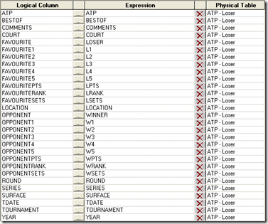
By doing this we make the Dimension logical table to have the universal information about a player & his opponent. It will take a while to understand this as this is the key in this modeling scenario. Next we map the individual logical table aliases to their corresponding Fact Tables.
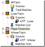
Not only this, we can use the same approach to provide more than one perspective of the data. For example, if you are analyzing football then you can give a Home/Away perspective in addition to Winner/Loser perspective. Also, the same approach above can be used for games where more than 2 teams are involved in a single game. For example, Formula 1, Athletics etc.
To test this, we start with Analyzing Top 5 Players Win record in the last 3 years
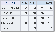
And if you look at the query generated, it will contain a universal perspective of all the 5 players above as Winners. So, only one Alias will be used.
select T30942.WINNER as c1,
     T30942.YEAR as c2,
     sum(case  when not T30942.LOSER is null then 1 else 0 end ) as c3
from
     ATP T30942 /* ATP - Winner */
where  ( T30942.WINNER in ('Del Potro J.M.', 'Djokovic N.', 'Federer R.', 'Murray A.', 'Nadal R.') )
group by T30942.WINNER, T30942.YEAR
order by c1, c2
Lets include the Loss Statistics as well and see the resulting query.
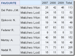
WITH
SAWITH0 AS (select sum(case  when not T30942.LOSER is null then 1 else 0 end ) as c1,
     T30942.WINNER as c2,
     T30942.YEAR as c3
from
     ATP T30942 /* ATP - Winner */
where  ( T30942.WINNER in ('Del Potro J.M.', 'Djokovic N.', 'Federer R.', 'Murray A.', 'Nadal R.') )
group by T30942.WINNER, T30942.YEAR),
SAWITH1 AS (select sum(case  when not T30972.LOSER is null then 1 else 0 end ) as c1,
     T30972.LOSER as c2,
     T30972.YEAR as c3
from
     ATP T30972 /* ATP - Loser */
where  ( T30972.LOSER in ('Del Potro J.M.', 'Djokovic N.', 'Federer R.', 'Murray A.', 'Nadal R.') )
group by T30972.LOSER, T30972.YEAR)
select distinct case  when SAWITH1.c2 is not null then SAWITH1.c2 when SAWITH0.c2 is not null then SAWITH0.c2 end  as c1,
     case  when SAWITH1.c3 is not null then SAWITH1.c3 when SAWITH0.c3 is not null then SAWITH0.c3 end  as c2,
     SAWITH0.c1 as c3,
     SAWITH1.c1 as c4
from
     SAWITH0 full outer join SAWITH1 On nvl(SAWITH0.c2 , 'q') = nvl(SAWITH1.c2 , 'q') and nvl(SAWITH0.c2 , 'z') = nvl(SAWITH1.c2 , 'z') and nvl(SAWITH0.c3 , 'q') = nvl(SAWITH1.c3 , 'q') and nvl(SAWITH0.c3 , 'z') = nvl(SAWITH1.c3 , 'z')
order by c1, c2
As you see BI EE will automatically make a sub-query join across both the aliases since we have measures coming in from 2 different fact tables. The join is done as both the fact measures conform to the common dimension. There are quite a few other interesting stats that one can derive out of this. Like for example, we would like to know the list of matches that Federer has lost in the last year and also the opponents & the courts.
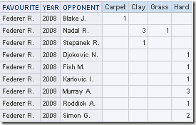
Interestingly he has lost to a total of 9 players. But Nadal & Murray have beaten him quite a few times more than other players. So, lets narrow this down further to see where Federer lost to Nadal & Murray

There are lots of other stats that we can accomplish out of this. I will stop here & will let FIFA, ATP etc notice this :-). Interestingly, in any major website there is not a lot of stats that are open for public. Only if we could have a live Web-Service giving us the results of each game & their stats, we can have even more interesting results for other sports (like what makes Usain Bolt faster than any other athlete!!! etc). But the point is BI EE can do these kind of statistical reporting pretty easily if modeled correctly in the repository.