Oracle BI EE 10.1.3.4.1 – Understanding Logical Calculations & Native DB Calculations – Repository Modeling

Venkatakrishnan J

Jan 15, 2010 • 7 min read

Ever wondered what is the actual difference between the logical calculated measures in the repository and the native DB calculated measures? I have had this question asked to me quite a few times in the recent past that i thought it made sense to create a separate blog entry for it. The difference between the 2 can turn out to be pretty significant and can even result in different numbers if not correctly used. Lets look at the differences between these 2 and how they together can provide excellent SQL Analytics capabilities in the repository.

Just to emphasize, logical calculated measures do not mean that the calculations will be done in the BI Server. Though it is possible in some cases that such logical calculations can be pushed to the BI Server layer, they have a completely different significance. Lets understand this through a couple of examples. Lets take the SH schema that gets installed as a sample schema in the Oracle database. Its a schema that contains 2 fact tables (SALES and COSTS) and set of dimension tables (PRODUCTS, PROMOTIONS, TIMES, CHANNELS & CUSTOMERS). Lets assume that SALES fact table has the following measures

AMOUNT_SOLD
AMOUNT_BUDGETED

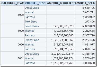
Now, for the sake of illustration, lets assume that the FACT table SALES has data way back from 1998 for the AMOUNT_SOLD measure. But the Budgeting process only started in 1999. So, for all the records in the SALES fact table the AMOUNT_BUDGETED would be null for the year 1998 as shown below.

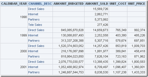
Along the same lines, lets assume that the COSTS fact table (or the COSTS tracking application) came into existence only in 1999. So, even the COSTS measures UNIT_PRICE and UNIT_COST will be null for the year 1998.

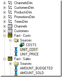
Also, to give you a perspective, since SALES and COSTS fact tables are at differing grains, they have been modeled as separate fact tables as shown below.

Lets start with a very simple requirement. No measures should be shown as nulls. All nulls should be replaced by zeroes. Seems pretty straight forward.

DB Calculation:

The most common way of doing this is, we go into the AMOUNT_BUDGETED, UNIT_PRICE & UNIT_COST measure in the LTS mapping and apply a formula in the mapping as shown below.

After making this change, lets go back to the report and see the result.

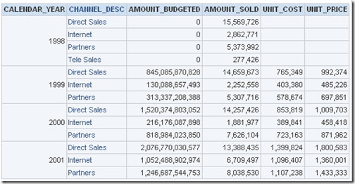
If you notice, the IFNULL is applied only on the AMOUNT_BUDGETED measure. The main reason behind this is, when you apply a calculation on a measure in the LTS mapping area, that will be applied only on existing rows. In our case, we have data combined from 2 different fact tables. In the case of AMOUNT_BUDGETED, the row for 1998 existed and it was a matter of the measure being NULL. But in the case of UNIT_COST and UNIT_PRICE the corresponding rows for the year 1998 do not even exist. Hence the application of IFNULL in the mapping layer at-least for this example is of no use. You can clearly understand this by looking at the actual SQL query fired.

WITH
SAWITH0 AS (select sum(T6428.AMOUNT_SOLD) as c1,
     sum(nvl(T6428.AMOUNT_BUDGETED , 0)) as c2,
     T6476.CALENDAR_YEAR as c3,
     T6294.CHANNEL_DESC as c4
from
     TIMES T6476,
     CHANNELS T6294,
     SALES T6428
where  ( T6294.CHANNEL_ID = T6428.CHANNEL_ID and T6428.TIME_ID = T6476.TIME_ID )
group by T6294.CHANNEL_DESC, T6476.CALENDAR_YEAR),
SAWITH1 AS (select sum(nvl(T6302.UNIT_PRICE , 0)) as c1,
     sum(nvl(T6302.UNIT_COST , 0)) as c2,
     T6476.CALENDAR_YEAR as c3,
     T6294.CHANNEL_DESC as c4
from
     TIMES T6476,
     CHANNELS T6294,
     COSTS T6302
where  ( T6294.CHANNEL_ID = T6302.CHANNEL_ID and T6302.TIME_ID = T6476.TIME_ID )
group by T6294.CHANNEL_DESC, T6476.CALENDAR_YEAR)
select distinct case  when SAWITH1.c3 is not null then SAWITH1.c3 when SAWITH0.c3 is not null then SAWITH0.c3 end  as c1,
     case  when SAWITH1.c4 is not null then SAWITH1.c4 when SAWITH0.c4 is not null then SAWITH0.c4 end  as c2,
     SAWITH0.c2 as c3,
     SAWITH0.c1 as c4,
     SAWITH1.c2 as c5,
     SAWITH1.c1 as c6
from
     SAWITH0 full outer join SAWITH1 On SAWITH0.c3 = SAWITH1.c3 and SAWITH0.c4 = SAWITH1.c4
order by c1, c2

As you see in the query above, the IFNULL is pushed only in the inner sub-queries. But the null in COST measures appear when the conforming dimension join happens – which is in the outer query. How do we push the IFNULL to the outer query.

Logical Calculations:

Lets introduce a Logical Calculated column for both UNIT_PRICE and UNIT_COST as shown below.

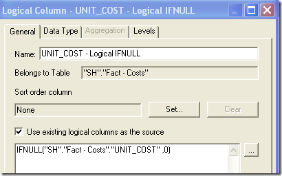
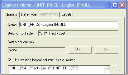
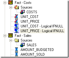
Lets include these 2 measures instead of the older measures in the report.

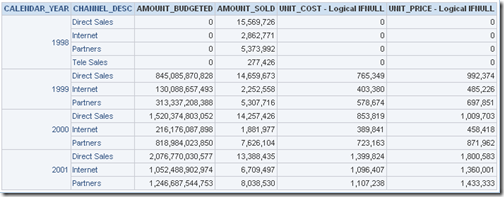
This has effectively converted the null cost measures to zero. If you look at the query below, you will notice that the outer query will have IFNULL(nvl in this case) clause on both the cost measures.

WITH
SAWITH0 AS (select sum(T6428.AMOUNT_SOLD) as c1,
     sum(nvl(T6428.AMOUNT_BUDGETED , 0)) as c2,
     T6476.CALENDAR_YEAR as c3,
     T6294.CHANNEL_DESC as c4
from
     TIMES T6476,
     CHANNELS T6294,
     SALES T6428
where  ( T6294.CHANNEL_ID = T6428.CHANNEL_ID and T6428.TIME_ID = T6476.TIME_ID )
group by T6294.CHANNEL_DESC, T6476.CALENDAR_YEAR),
SAWITH1 AS (select sum(nvl(T6302.UNIT_PRICE , 0)) as c1,
     sum(nvl(T6302.UNIT_COST , 0)) as c2,
     T6476.CALENDAR_YEAR as c3,
     T6294.CHANNEL_DESC as c4
from
     TIMES T6476,
     CHANNELS T6294,
     COSTS T6302
where  ( T6294.CHANNEL_ID = T6302.CHANNEL_ID and T6302.TIME_ID = T6476.TIME_ID )
group by T6294.CHANNEL_DESC, T6476.CALENDAR_YEAR)
select distinct case  when SAWITH1.c3 is not null then SAWITH1.c3 when SAWITH0.c3 is not null then SAWITH0.c3 end  as c1,
     case  when SAWITH0.c4 is not null then SAWITH0.c4 when SAWITH1.c4 is not null then SAWITH1.c4 end  as c2,
     SAWITH0.c2 as c3,
     SAWITH0.c1 as c4,
     nvl(SAWITH1.c2 , 0) as c5,
     nvl(SAWITH1.c1 , 0) as c6
from
     SAWITH0 full outer join SAWITH1 On SAWITH0.c3 = SAWITH1.c3 and SAWITH0.c4 = SAWITH1.c4
order by c1, c2

Some might argue that IFNULL in the mapping (db calculation) is redundant for the AMOUNT_BUDGETED measure as we can have the same effect by using a logically calculated AMOUNT_BUDGETED measure(like what we did for UNIT_COST & UNIT_PRICE). This argument is true for this case. But database calculations are always preferred over Logical Calculations unless the calculation cannot be pushed into the database. Lets see why.

Logical Calculation & DB Calculation:

For example, lets create 2 measures which are basically derived measures calculating the difference between AMOUNT_SOLD and AMOUNT_BUDGETED. Variance is a measure where the calculation of AMOUNT_SOLD – AMOUNT_BUDGETED is in the LTS mapping layer. Logical Variance is a measure where the same calculation is in the Logical calculation section as shown below

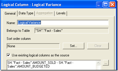
Lets create a report containing both the measures separately and look at the SQL queries fired.

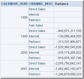
select T6476.CALENDAR_YEAR as c1,
     T6294.CHANNEL_DESC as c2,
     sum(T6428.AMOUNT_SOLD - T6428.AMOUNT_BUDGETED) as c3
from
     TIMES T6476,
     CHANNELS T6294,
     SALES T6428
where  ( T6294.CHANNEL_ID = T6428.CHANNEL_ID and T6428.TIME_ID = T6476.TIME_ID )
group by T6294.CHANNEL_DESC, T6476.CALENDAR_YEAR
order by c1, c2

This query is as expected. But lets create the same report using the Logical Calculated column.

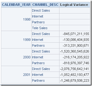
The results are the same. But if you look at the query fired

WITH
SAWITH0 AS (select sum(T6428.AMOUNT_BUDGETED) as c1,
     sum(T6428.AMOUNT_SOLD) as c2,
     T6476.CALENDAR_YEAR as c3,
     T6294.CHANNEL_DESC as c4
from
     TIMES T6476,
     CHANNELS T6294,
     SALES T6428
where  ( T6294.CHANNEL_ID = T6428.CHANNEL_ID and T6428.TIME_ID = T6476.TIME_ID )
group by T6294.CHANNEL_DESC, T6476.CALENDAR_YEAR)
select distinct SAWITH0.c3 as c1,
     SAWITH0.c4 as c2,
     SAWITH0.c2 - SAWITH0.c1 as c3
from
     SAWITH0
order by c1, c2

you will notice that there is a significant change in the query. There is an un-necessary inline view that BI Server creates. This is absolutely not desired as all that you are doing is a simple difference in measure calculation at-least for this use-case. In effect, the point is while designing a model for reporting we need to ensure that the calculations are pushed at the right places to derive maximum performance. Both type of calculations complement each other very well though. In fact, in some complex scenarios we can control the order of joins made across the tables by mixing the database and logical calculations. Well, that is a topic for another blog entry altogether!!! Though the use cases above are pretty simple, the same logic can be applied for complex scenarios (like assume a requirement where DB calculation happens at a lower level but the Logical calculation happens at another level). This way we can tweak how our SQL queries are constructed by the BI Server.

Sign up for more like this.