ETL Offload with Spark and Amazon EMR - Part 2 - Code development with Notebooks and Docker
In the previous article I gave the background to a project we did for a client, exploring the benefits of Spark-based ETL processing running on Amazon's Elastic Map Reduce (EMR) Hadoop platform. The proof of concept we ran was on a very simple requirement, taking inbound files from a third party, joining to them to some reference data, and then making the result available for analysis. The primary focus was proving the end-to-end concept, with future iterations focussing on performance and design optimisations.
Here we'll see how I went about building up the ETL process.
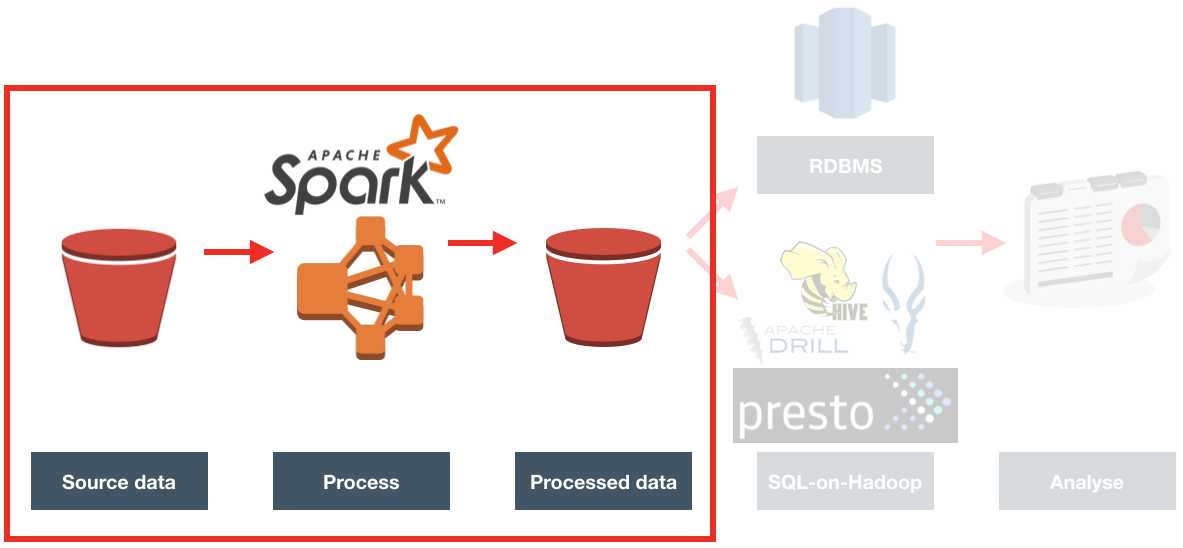
Processing Overview
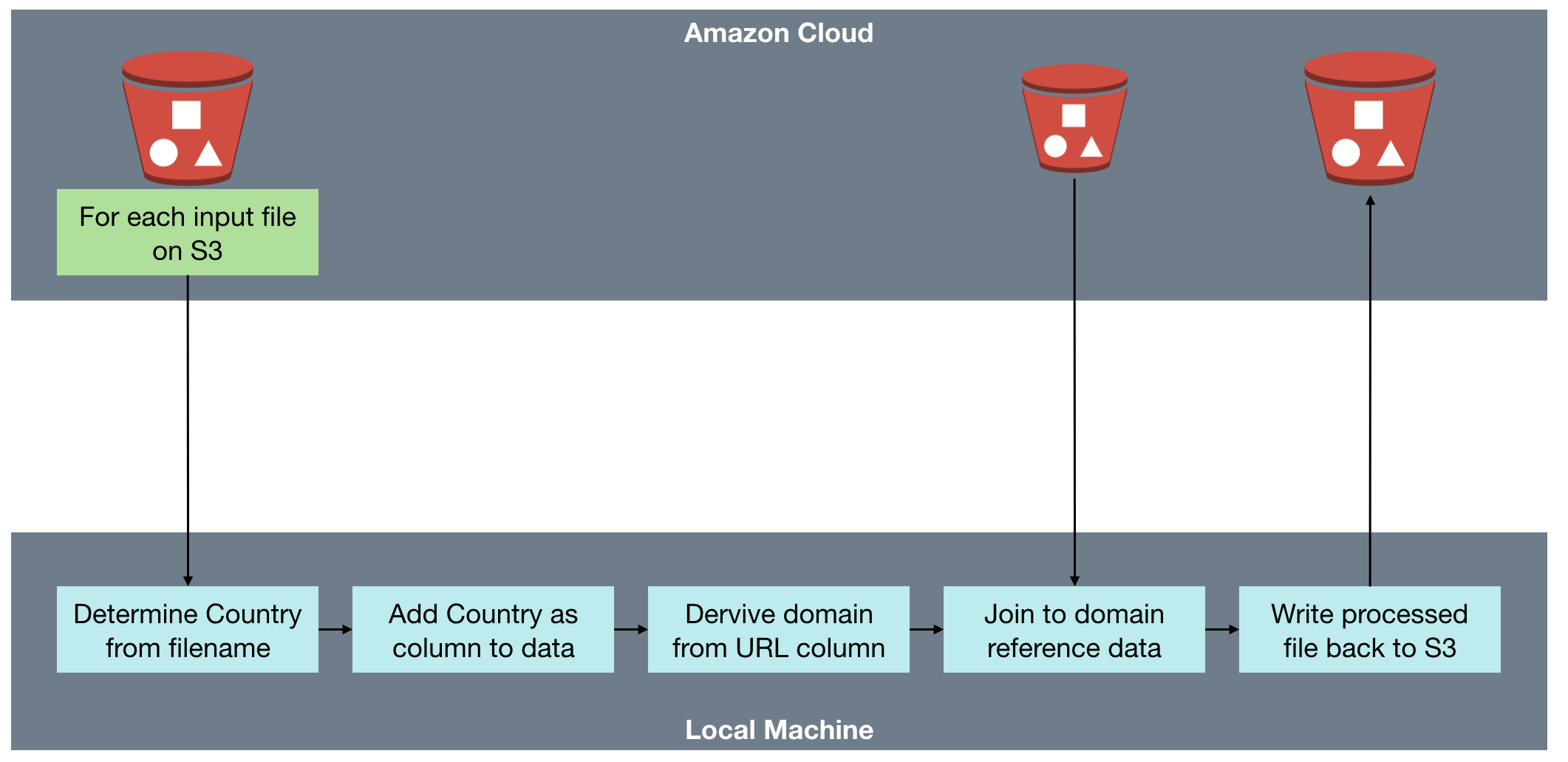
The processing needed to iterate over a set of files in S3, and for each one:
- Loads the file from S3
- Determines region from filename, and adds as column to data
- Deduplicates it
- Writes duplicates to separate file
- Loads sites reference data
- Extracts domain from URL string
- Joins facts with sites on domain
- Writes resulting file to S3
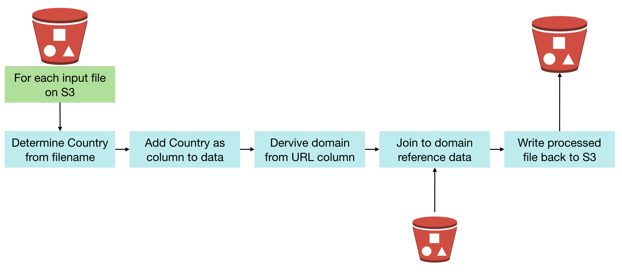
Once the data is processed and landed back to S3, we can run analytics on it. See subsequent articles for discussion of Redshift vs in-place querying with tools such as Presto.
Ticking All The Cool-Kid Boxes - Spark AND Notebooks AND Docker!
Whilst others in Rittman Mead have done lots of work with Spark, I myself was new to it, and needed a sandpit in which I could flail around without causing any real trouble. Thus I set up a nice self-contained development environment on my local machine, using Docker to provision and host it, and Jupyter Notebooks as the interface.
Notebooks
In a world in which it seems that there are a dozen cool new tools released every day, Interactive Notebooks are for me one of the most significant of recent times for any developer. They originate in the world of data science, where taking the 'science' bit at its word, data processing and exploration is written in a self-documenting manner. It makes it possible to follow how and why code was written, what the output at each stage was -- and to run it yourself too. By breaking code into chunks it makes it much easier to develop as well, since you can rerun and perfect each piece before moving on.
Notebooks are portable, meaning that you can work with them in one system, and then upload them for others to learn from and even import to run on their own systems. I've shared a simplified version of the notebook that I developed for this project on gist here, and you can see an embedded version of it at the end of this article.
The two most common are Apache Zeppelin, and Jupyter Notebooks (previously known as iPython Notebooks). Jupyter is the one I've used previously, and stuck with again here. To read more about notebooks and see them in action, see my previous blog posts here and here.
Docker
Plenty's been written about Docker. In a nutshell, it is a way to provision and host a set of self-contained software. It takes the idea of a virtual machine (such as VMWare, or VirtualBox), but without having to install an OS, and then the software, and then configure it all yourself. You simply take a "Dockerfile" that someone has prepared, and run it. You can create copies, or throwaway and start again, from a single command. I ran Docker on my Mac through Kitematic, and natively on my home server.
There are prebuilt Docker configuration files for lots of software (including Oracle and OBIEE!), and I found one that includes Spark, PySpark, and Jupyter - perfect!
To launch it, you simply enter:
docker run -d -p 18888:8888 jupyter/all-spark-notebook
This downloads all the necessary Docker files etc - you don't need anything local first, except Docker.
I ran it with an additional flag, -v, configuring it to use a folder on my local machine to store the work that I created. By default all files reside within the Docker image itself - and get deleted when you delete the Docker instance.
docker run -d -p 18888:8888 -v /Users/rmoff/all-spark-notebook:/home/jovyan/work jupyter/all-spark-notebook
You can also run the container with an additional flag, GRANT_SUDO, so that the guest user can run sudo commands within it. To do this include -e GRANT_SUDO=yes --user root:
docker run -d -p 18888:8888 -e GRANT_SUDO=yes --user root -v /Users/rmoff/all-spark-notebook:/home/jovyan/work jupyter/all-spark-notebook
With the docker container running, you can access Jupyter notebooks on the port exposed in the command used to launch it (18888)
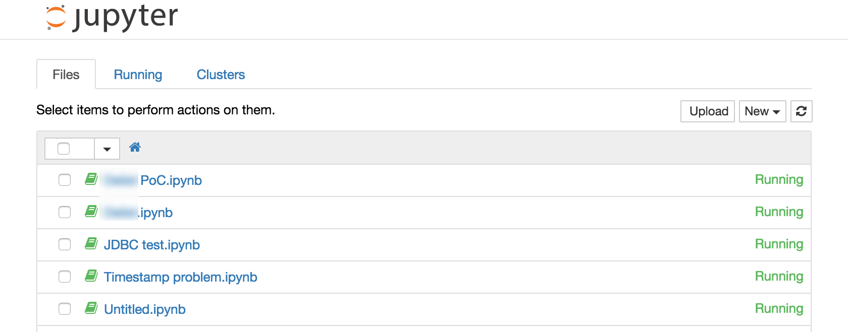
Getting Started with Jupyter
From Jupyter's main page you can see the files within the main folder (see above for how you can map this to a local folder on the machine hosting Docker). Using the New menu in the top-right you can create:
- Folders and edit Text files
- A terminal
- A notebook, running under one of several different 'Kernels' (host interpreters and environments)
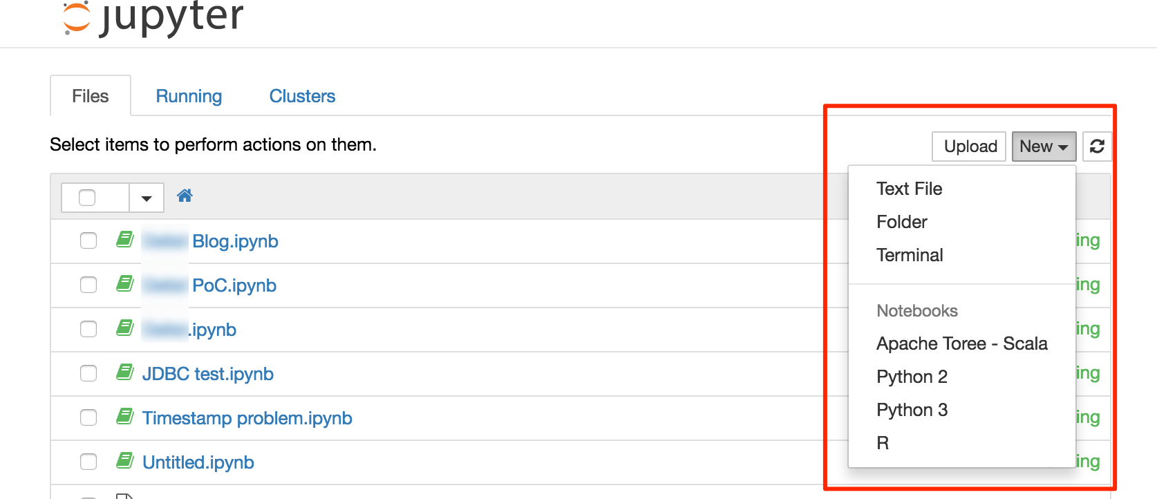
The ability to run a terminal from Jupyter is very handy - particularly on Docker. Docker by its nature isn't really designed for interaction within the container itself. It's the point of Docker in a way, that it provisions and configures all the software for you. You can use Docker to run a bash shell directly, but it's more fiddly than just using the Jupyer Terminal.
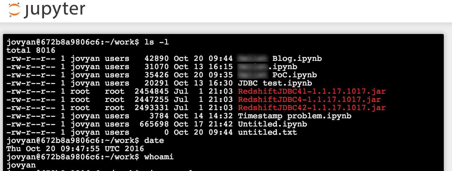
I used a Python 2 notebook for my work; with this Docker image you also have the option of Python 3, Scala, and R.

Developing the Spark job
With my development environment up and running, I set to writing the Spark job. Because I'm already familiar with Python I took advantage of PySpark. Below I describe the steps in the processing and how I achieved them.
Environment Preparation
Define AWS parameters:
access_key='XXXXXXXXXXXXXXXXXX
secret='YYYYYYYYYYYYYYYYY'
bucket_name='foobar-bucket'
Set up the PySpark environment, including necessary JAR files for accessing S3 from Spark:
import os
os.environ['AWS_ACCESS_KEY_ID'] = access_key
os.environ['AWS_SECRET_ACCESS_KEY'] = secret
os.environ['PYSPARK_PYTHON'] = '/usr/bin/python2'
os.environ['PYSPARK_SUBMIT_ARGS'] = '--packages org.apache.hadoop:hadoop-aws:2.7.1,com.amazonaws:aws-java-sdk-pom:1.10.34,com.databricks:spark-csv_2.11:1.3.0 pyspark-shell'
Create a spark context:
import pyspark
sc = pyspark.SparkContext('local[*]')
sqlContext = pyspark.SQLContext(sc)
Import Python libraries
from pyspark.sql.functions import udf
from pyspark.sql.functions import lit
import boto
from urlparse import urlsplit
Note that to install python libraries not present on the Docker image (such as boto, which is used for accessing AWS functionality from within Python) you can run from a Jupyter Terminal:
/opt/conda/envs/python2/bin/pip install boto
On other platforms the path to pip will vary, but the install command is the same
Loading Data from S3
The source data comes from an S3 "bucket", on which there can be multiple "keys". Buckets and keys roughly translate to "disk drive" and "file".
We use the boto library to interact with S3 to find a list of files ('keys') matching the pattern of source files that we want to process.
Connect to the bucket
conn_s3 = boto.connect_s3()
bucket = conn_s3.get_bucket(bucket_name)
Iterate over the bucket contents
This bit would drive iterative processing over multiple input files; for now it just picks the last file on the list (acme_file getting set on each iteration and so remaining set after the loop)
contents=bucket.list(prefix='source_files/')
for f in contents:
    print f.name
    print f.size
    acme_file = f.name
print "\n\n--\nFile to process: %s" % acme_file
Read the CSV from S3 into Spark dataframe
The Docker image I was using was running Spark 1.6, so I was using the Databricks CSV reader; in Spark 2 this is now available natively. The CSV file is loaded into a Spark data frame. Note that Spark is reading the CSV file directly from a S3 path.
full_uri = "s3n://{}/{}".format(bucket_name, acme_file)
print full_uri
s3n://foobar-bucket/source_files/acme_GB_20160803_100000.csv
acme_df = sqlContext.read.load(full_uri,
                                  format='com.databricks.spark.csv',
                                  header='true',
                                  inferSchema='true')

acme_df.printSchema()
root
 |-- product: string (nullable = true)
 |-- product_desc: string (nullable = true)
 |-- product_type: string (nullable = true)
 |-- supplier: string (nullable = true)
 |-- date_launched: timestamp (nullable = true)
 |-- position: string (nullable = true)
 |-- url: string (nullable = true)
 |-- status: string (nullable = true)
 |-- reject_reason: string (nullable = true)
The above shows the schema of the dataframe; Spark has infered this automagically from the column headers (for the column names), and then the data types within (note that it has correctly detected a timestamp in the date_launched column)
Add country column to data frame
The filename of the source data includes a country field as part of it. Here we use this regular expression to extract it:
filename=os.path.split(acme_file)[1]
import re
m=re.search('acme_([^_]+)_.+$', filename)
if m is None:
    country='NA'
else:
    country=m.group(1)

print "Country determined from filename '%s' as : %s" % (filename,country)
Country determined from filename 'acme_GB_20160803_100000.csv' as : GB
With the country stored in a variable, we add it as a column to the data frame:
Note that the withColumn function requires a Column value, which we create here using the PySpark lit function that was imported earlier on.
acme_df=acme_df.withColumn('country',lit(country))

acme_df.printSchema()
root
 |-- product: string (nullable = true)
 |-- product_desc: string (nullable = true)
 |-- product_type: string (nullable = true)
 |-- supplier: string (nullable = true)
 |-- date_launched: timestamp (nullable = true)
 |-- position: string (nullable = true)
 |-- url: string (nullable = true)
 |-- status: string (nullable = true)
 |-- reject_reason: string (nullable = true)
 |-- country: string (nullable = false)
Note the new column added to the end of the schema.
Deduplication
Now that we've imported the file, we need to deduplicate it to remove entries with the same value for the url field. Here I'm created a second dataframe based on a deduplication of the first, using the PySpark native function dropDuplicates:
acme_deduped_df = acme_df.dropDuplicates(['url'])
For informational purposes we can see how many records are in the two dataframes, and determine how many duplicates there were:
orig_count = acme_df.count()
deduped_count = acme_deduped_df.count()
print "Original count: %d\nDeduplicated count: %d\n\n" % (orig_count,deduped_count)
print "Number of removed duplicate records: %d" % (orig_count - deduped_count)
Original count: 97974
Deduplicated count: 96706


Number of removed duplicate records: 1268
Deriving Domain from URL
One of the sets of reference data is information about the site on which the product was viewed. To bring these sets of attributes into the main dataset we join on the domain itself. To perform this join we need to derive the domain from the URL. We can do this using the python urlsplit library, as seen in this example:
sample_url = 'https://www.rittmanmead.com/blog/2016/08/using-apache-drill-with-obiee-12c/'

print sample_url
print urlsplit(sample_url).netloc
https://www.rittmanmead.com/blog/2016/08/using-apache-drill-with-obiee-12c/
www.rittmanmead.com
We saw above that to add a column to the dataframe the withColumn function can be used. However, to add a column that's based on another (rather than a literal, which is what the country column added above was) we need to use the udf function. This generates the necessary Column field based on the urlsplit output for the associated url value.
First we define our own function which simply applies urlsplit to the value passed to it
def getDomain(value):
    return urlsplit(value).netloc
and then a UDF based on it:
udfgetDomain = udf(getDomain)
Finally, apply this to a third version of the dataframe:
acme_deduped_df_with_netloc = acme_deduped_df.withColumn("netloc", udfgetDomain(acme_deduped_df.url))
Joining to Second Dataset
Having preparing the primary dataset, we'll now join it to the reference data. The source of this is currently an Oracle database. For simplicity we're working with a CSV dump of the data, but PySpark supports the option to connect to sources with JDBC so we could query it directly if required.
First we import the sites reference data CSV:
sites_file = "s3n://{}/{}".format('foobar-bucket', 'sites.csv')
sites_df = sqlContext.read.load(sites_file,
                                  format='com.databricks.spark.csv',
                                  header='true',
                                  inferSchema='true')
Then some light data cleansing with the filter function to remove blank SITE entries, and blank SITE_RETAIL_TYPE entries:
sites_pruned_df = sites_df.filter("NOT (SITE ='' OR SITE_RETAIL_TYPE = '')")
Now we can do the join itself. This joins the original dataset (acme_deduped_df_with_netloc) with the sites reference data (sites_pruned_df), using a left outer join.
merged_df = acme_deduped_df_with_netloc.join(sites_pruned_df,acme_deduped_df_with_netloc.netloc == sites_pruned_df.SITE, 'left_outer')
Using the filter function and show we can inspect the dataset for matches, and misses:
First 10 matched:
merged_df.filter(merged_df.ID.isNotNull()).select('date_launched','url','netloc','ID','SITE','SITE_RETAIL_TYPE').show(10)
First 10 unmatched:
merged_df.filter(merged_df.ID.isNull()).select('date_launched','url','netloc','ID','SITE','SITE_RETAIL_TYPE').show(10)
Write Back to S3
The finished dataset is written back to S3. As before, we're using the databricks CSV writer here but in Spark 2 would be doing it natively:
acme_enriched_filename='acme_enriched/%s' % filename.replace('.csv','')
full_uri = "s3n://{}/{}".format(bucket_name, acme_enriched_filename)
print 'Writing enriched acme data to %s' % full_uri
merged_df.write.save(path=full_uri,
                     format='com.databricks.spark.csv',
                     header='false',
                     nullValue='null',
                     mode='overwrite')
Summary
With the above code written, I could process input files in a couple of minutes per 30MB file. Bear in mind two important constraints to this performance:
-
I was working with data residing up in the Amazon Cloud, with the associated network delay in transferring to and from it
-
The processing was taking place on a single node Spark deployment (on my laptop, under virtualisation), rather than the multiple-node configuration typically seen.
The next steps, as we'll see in the next article, were to port this code up to Amazon Elastic Map Reduce (EMR). Stay tuned!
Footnote: Notebooks FTW!
(FTW)
Whilst I've taken the code and written it out above more in the form of a blog post, I could have actually just posted the Notebook itself, and it wouldn't have needed much more explanation. Here it is, along with some bonus bits on using S3 from python:
