OCI Data Flow: ETL with Apache Spark in the Cloud

About OCI Data Flow
Oracle Cloud Infrastructure (OCI) Data Flow is a managed service for running Apache Spark applications, promising simplified infrastructure management, development, and deployment. Initial impressions suggest it delivers on this promise, showcasing an elegant approach to certain tasks.
To assess OCI Data Flow's capabilities, a test was conducted involving the extraction of Orders data from various flat file sources, subsequent analysis, and loading into an Oracle Autonomous Data Warehouse (ADW) table. This evaluation focuses on the technical aspects, omitting details regarding Oracle Cloud Identity and Access Management policy setup.
The Setup
Three flat files served as data sources for this evaluation:
- Customers (CSV): Contains customer identification details alongside their names and addresses.
"customer_id","first_name","last_name","address"
"1","James","Smith","123 Main Street, Anytown, CA 12345, USA"
"2","Maria","Garcia","456 Elm Avenue, Anytown, CA 12345, USA"
"3","David","Brown","789 Oak Street, Anytown, CA 12345, USA"
"4","Emily","Jones","101 Pine Lane, Anytown, CA 12345, USA"
"5","Michael","Johnson","202 Cedar Road, Anytown, CA 12345, USA"
...- Products (JSON): Structured as a JSON array of objects, each detailing individual product attributes like name, description, class, and manufacturer.
[
  {
    "product_id": 1,
    "product_name": "Laptop X1 Pro",
    "product_description": "High-performance laptop with a 15-inch 4K display.",
    "product_class": "Electronics",
    "product_subclass": "Computers & Laptops",
    "product_manufacturer_name": "TechCo"
  },
  {
    "product_id": 2,
    "product_name": "Smartphone Z5",
    "product_description": "Latest smartphone with a triple camera system.",
    "product_class": "Electronics",
    "product_subclass": "Mobile Phones",
    "product_manufacturer_name": "MobileTech"
  },
  {
    "product_id": 3,
    "product_name": "SneakerAir Max",
    "product_description": "Comfortable running shoes with air cushioning.",
    "product_class": "Apparel",
    "product_subclass": "Footwear",
    "product_manufacturer_name": "SportWear"
  },
...
]- Orders (Parquet): A binary file format, viewed through a Parquet viewer, containing information on customer orders, such as quantities and prices.

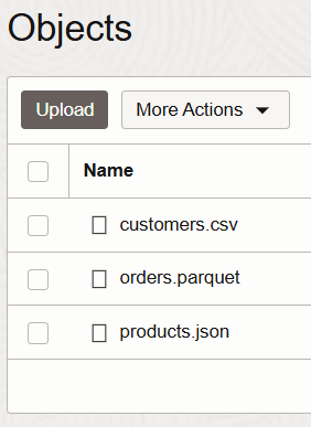
The initial step involved deploying the three flat files to an OCI Object Storage bucket named dftest-managed-table-bucket. This process, encompassing the creation of the bucket and subsequent file uploads, was completed within a minute.

Two additional OCI Object Storage buckets were created for supplementary purposes:
- dftest-logs: Intended for storing log files generated during the data flow process.
- dftest-python-code: Designed to hold the PySpark script responsible for orchestrating the data extraction, transformation, and loading (ETL) operations.
The Code
For this demonstration, a single Python script was used. (A typical PySpark deployment would include several scripts and non-standard libraries.) It begins by reading DataFrames from the flat files located in the designated OCI Object Storage bucket. The script leverages PySpark's built-in functions (spark.read.csv, spark.read.json, spark.read.parquet) to efficiently ingest data from the CSV, JSON, and Parquet files respectively. The show() and printSchema() methods are then employed to display the first few rows of each DataFrame and their corresponding schema, verifying successful data loading and inferring data types.
    customers_csv_file_path = "oci://dftest-managed-table-bucket@xxxxxxxx/customers.csv"
    products_json_file_path = "oci://dftest-managed-table-bucket@xxxxxxxx/products.json"
    orders_parquet_file_path = "oci://dftest-managed-table-bucket@xxxxxxxx/orders.parquet"

    customers_df = spark.read.csv(customers_csv_file_path, header=True, inferSchema=True)
    customers_df.show(5)
    customers_df.printSchema()

    products_df = spark.read.json(products_json_file_path, multiLine=True)
    products_df.show(5)
    products_df.printSchema()

    orders_df = spark.read.parquet(orders_parquet_file_path)
    orders_df.show(5)
    orders_df.printSchema()
The console output demonstrates the successful ingestion of data into Spark DataFrames. The JSON, Parquet, and CSV parsers efficiently processed the source files, requiring minimal configuration.
The show() method reveals the first five rows of each DataFrame.
The printSchema() method outputs the inferred schema for each DataFrame, confirming accurate identification of data types. Notably, all fields are recognized as nullable, accommodating potential missing values.
This output verifies the readiness of the data for subsequent analysis and processing within the Spark environment.
|customer_id|first_name|last_name|             address|
+-----------+----------+---------+--------------------+
|          1|     James|    Smith|123 Main Street, ...|
|          2|     Maria|   Garcia|456 Elm Avenue, A...|
|          3|     David|    Brown|789 Oak Street, A...|
|          4|     Emily|    Jones|101 Pine Lane, An...|
|          5|   Michael|  Johnson|202 Cedar Road, A...|
+-----------+----------+---------+--------------------+
only showing top 5 rows

root
 |-- customer_id: integer (nullable = true)
 |-- first_name: string (nullable = true)
 |-- last_name: string (nullable = true)
 |-- address: string (nullable = true)

+-------------+--------------------+----------+-------------------------+-------------------+-------------------+
|product_class| product_description|product_id|product_manufacturer_name|       product_name|   product_subclass|
+-------------+--------------------+----------+-------------------------+-------------------+-------------------+
|  Electronics|High-performance ...|         1|                   TechCo|      Laptop X1 Pro|Computers & Laptops|
|  Electronics|Latest smartphone...|         2|               MobileTech|      Smartphone Z5|      Mobile Phones|
|      Apparel|Comfortable runni...|         3|                SportWear|     SneakerAir Max|           Footwear|
|   Appliances|Automatic coffee ...|         4|                 HomeBrew|Coffee Maker Deluxe| Kitchen Appliances|
|  Electronics|Noise-cancelling ...|         5|                SoundWave|Wireless Headphones|    Audio Equipment|
+-------------+--------------------+----------+-------------------------+-------------------+-------------------+
only showing top 5 rows

root
 |-- product_class: string (nullable = true)
 |-- product_description: string (nullable = true)
 |-- product_id: long (nullable = true)
 |-- product_manufacturer_name: string (nullable = true)
 |-- product_name: string (nullable = true)
 |-- product_subclass: string (nullable = true)

+-----------+----------+-------------+--------------+
|customer_id|product_id|units_ordered|price_per_unit|
+-----------+----------+-------------+--------------+
|          1|         1|            5|         55.53|
|          1|         2|            2|         18.77|
|          1|         3|            2|         64.99|
|          1|         4|            4|         81.25|
|          1|         5|            4|         59.16|
+-----------+----------+-------------+--------------+
only showing top 5 rows

root
 |-- customer_id: long (nullable = true)
 |-- product_id: long (nullable = true)
 |-- units_ordered: long (nullable = true)
 |-- price_per_unit: double (nullable = true)
Following the successful data ingestion and type recognition, the subsequent analysis aimed to generate a simple sales business intelligence (BI) report. This entailed:
- Joining the three datasets: Merging customer, product, and order information to create a unified view of sales transactions.
- Aggregation: Calculating the total units ordered and total order price, grouped by product class and subclass.
- Ranking: Identifying the top 10 products based on their total order price.
Two approaches were explored for creating the sales analysis:
- Spark DataFrame API: This method utilises the DataFrame API's chainable functions to join and analyse the datasets. While verbose, it provides clear step-by-step logic, appealing to those with a software engineering background.
- Spark SQL: This approach leverages Spark's SQL interface by creating temporary views for the DataFrames. The analysis is then expressed as a standard ANSI SQL query, involving joins, aggregations, sorting, and limiting, mirroring operations familiar to SQL practitioners.
Both approaches yield identical results but differ in their coding styles and underlying mechanisms. Choosing between them is a matter of personal preference and expertise.
The Spark DataFrame API approach:
    orders_detail_df = (orders_df
                 .join(customers_df, on="customer_id", how="inner")     # join customers to orders
                 .join(products_df, on="product_id", how="inner")       # join products to orders
                 .select(
                    col("first_name").alias("customer_first_name"),
                    col("last_name").alias("customer_last_name"),
                    col("product_class"),
                    col("product_subclass"),
                    col("product_name"),
                    col("units_ordered"),
                    col("price_per_unit")
                 )
                 .withColumn("order_price", col("units_ordered") * col("price_per_unit"))
                 )

    orders_summary_df = (orders_detail_df
    .groupBy("product_class", "product_subclass").agg(
        sum("units_ordered").alias("total_units_ordered"),
        sum("order_price").alias("total_price")
    )
    .orderBy(col("total_price").desc())
    .limit(10)
    )
The Spark SQL approach:
    orders_df.createOrReplaceTempView("orders")
    customers_df.createOrReplaceTempView("customers")
    products_df.createOrReplaceTempView("products")

    sql_grouping_query = """
    SELECT
        product_class,
        product_subclass,
        SUM(units_ordered) AS total_units_ordered,
        SUM(units_ordered * price_per_unit) AS total_price
    FROM
        orders
        INNER JOIN customers ON orders.customer_id = customers.customer_id
        INNER JOIN products ON orders.product_id = products.product_id
    GROUP BY
        product_class,
        product_subclass
    ORDER BY total_price DESC
    LIMIT 10
    """

    orders_summary_sql_df = spark.sql(sql_grouping_query)
Both approaches produce the same result:
+-----------------+--------------------+-------------------+------------------+
|    product_class|    product_subclass|total_units_ordered|       total_price|
+-----------------+--------------------+-------------------+------------------+
|      Electronics|Cameras & Photogr...|                627| 35220.56017589569|
|          Apparel|          Activewear|                592|31161.999968528748|
|      Electronics|     Audio Equipment|                405| 22872.63992023468|
|          Apparel|            Footwear|                407| 22199.12000465393|
|Sports & Outdoors|      Yoga & Pilates|                220|13502.029949188232|
|      Electronics|    Drones & RC Toys|                226|13496.760019302368|
|Sports & Outdoors|        Water Sports|                221|13107.650062561035|
|Sports & Outdoors|             Cycling|                223| 13105.36001777649|
|       Appliances|  Kitchen Appliances|                224|12381.399991989136|
| Travel & Luggage|           Backpacks|                211|11986.040004730225|
+-----------------+--------------------+-------------------+------------------+

root
 |-- product_class: string (nullable = true)
 |-- product_subclass: string (nullable = true)
 |-- total_units_ordered: long (nullable = true)
 |-- total_price: double (nullable = true)
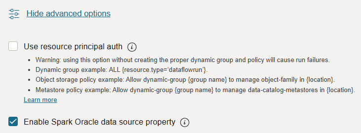
The culminating task involved writing the resulting DataFrame into an Oracle Autonomous Data Warehouse (ADW) table. Traditionally, accessing ADW necessitates the use of an Oracle database wallet, often presenting a challenge due to the requirement of deploying it on all executor nodes (wallets have to be local to the executor - a URL to an OCI Bucket will not suffice). However, a more streamlined approach exists within OCI Data Flow.
An easily-overlooked checkbox within the advanced section of OCI Data Flow's application configuration unlocks simplified wallet usage. Enabling this option not only provides access to Oracle JDBC drivers without manual packaging, but also handles wallet deployment to executor nodes automatically. Furthermore, when using ADW, even wallet management becomes unnecessary, requiring only the ADW database OCID for seamless integration.

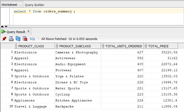
Returning to the PySpark script, the final step involved writing the orders_summary_sql_df DataFrame, resulting from the analysis, into the pre-existing "orders_summary" table within the provisioned ADW database.
    options = {
        "adbId": "ocid1.autonomousdatabase.oc1.uk-london-1.xxxxxxxxxxxxxxxxxxxxxxxxxxxxxxxxxxxxxxxxxxxxxxx",
        "dbtable": "orders_summary",
        "user": "USER_NAME",
        "password": "PASSWORD",
    }

    (orders_summary_sql_df
     .write
     .format("oracle")
     .options(**options)
     .mode("append")
     .save()
     )
The provided code snippet demonstrates the simplicity of this process using the enabled advanced configuration. By specifying the adbId (ADW database OCID), dbtable (target table name), and user credentials, the DataFrame is effortlessly written into the database without any explicit wallet handling.
This streamlined approach, achieved with approximately 50 lines of Python code, highlights the efficiency of OCI Data Flow. The script seamlessly integrates data extraction, transformation using SQL, and loading into the database, showcasing the platform's potential for concise and effective data pipeline development.
We can verify the outcome by querying the orders_summary table:

Challenges
In the example script, database credentials are provided in plain text. In a production environment, storing sensitive information like passwords in OCI Vault is best practice. However, accessing OCI Vault Secrets from Data Flow scripts is not straightforward and requires the oci Python library. When attempting to import the oci library in the Data Flow script (without having packaged it with the script), the following error occurs:
ModuleNotFoundError: No module named 'oci'
It's assumed that Oracle would provide standard libraries like 'oci' within the Data Flow environment. Despite this issue, the overall experience prototyping data processes with OCI Data Flow has been positive, demonstrating the service's potential.
Conclusion
The benefits of cloud computing for CRM systems and relational databases are well established. It's arguable that cloud computing is even more advantageous for distributed computing platforms like Apache Spark. The ability to dynamically allocate resources and scale executor nodes on demand is a key strength of cloud environments. This suggests that OCI Data Flow could have significant potential in this space.
