Data Lineage Analysis with Python and NetworkX

Use Network Graphs for Data Analysis
Python is one of the most capable and flexible data analysis tools out there. The data to be analysed comes in different formats and with different requirements for analysis. Some data is best represented and analysed as a network graph. A good example of that is data lineage.
Data lineage is the process of tracking the origin, transformations, and movement of data throughout its lifecycle within a data system, typically including its journey from the source database through any ETL processes, to reports, and even to the end users who access the data.
Data lineage can be effectively represented within a normalised relational database. However, comprehensive analysis of this lineage, particularly within a large-scale enterprise data system and when requiring traversal of the entire lineage (rather than a targeted search), may encounter significant performance challenges. (I have encountered such challenges first-hand in my experience.)
To select the most appropriate technology, organizations may consider robust graph database solutions such as Neo4j or Oracle Graph for large-scale projects. However, for smaller initiatives, utilising Python with its NetworkX library can provide a streamlined and efficient approach for constructing and analysing network graphs.
Lineage Analysis - a Simple Example
The Task
Let us look at a lineage analysis example: We have a relational database containing columns of sensitive data. We also have reports referencing these columns. In addition to that, we have end users, each with a list of reports they have accessed lately (or alternatively - a list of reports they have access to). Our goal is simple: for each sensitive column, we want to identify the users who have (or can) accessed it.
In a typical enterprise system, with potentially thousands of database fields, intricate ETL processes, numerous reports, and a large user base, data lineages can become extremely complex. The aforementioned analysis, requiring traversal of all sensitive columns, can be computationally intensive and may take hours or even days to complete if the chosen technology for analysis is not carefully considered.
The Source Data
Our data lineage is represented by 3 JSON files:
Database
Database content is a 3-level hierarchy with schemas, tables and columns, some of which are designated as sensitive.
{
  "database_schemas": [
    {
      "name": "Sales",
      "tables": [
        {
          "name": "Orders",
          "columns": [
            { "name": "OrderID", "sensitive": false },
            { "name": "CustomerID", "sensitive": false },
            { "name": "OrderDate", "sensitive": false },
            { "name": "TotalAmount", "sensitive": true }
          ]
        },
        {
          "name": "Customers",
          "columns": [
            { "name": "CustomerID", "sensitive": false },
            { "name": "FirstName", "sensitive": false },
            { "name": "LastName", "sensitive": false },
            { "name": "EmailAddress", "sensitive": true },
            { "name": "PhoneNumber", "sensitive": true },
            { "name": "BirthDate", "sensitive": false },
            { "name": "Gender", "sensitive": false },
            { "name": "City", "sensitive": false },
            { "name": "State", "sensitive": false }
          ]
        },
...
      ]
    },
...
  ]
}
Reports
Here we have reports consisting of fields, which reference one or many database columns.
{
  "reports": [
    {
      "name": "Sales Summary",
      "report_fields": [
        { "name": "Total Sales", "source_columns": ["Sales.Orders.TotalAmount"] },
        { "name": "Number of Orders", "source_columns": ["Sales.Orders.OrderID"] },
        { "name": "Average Order Value", "source_columns": ["Sales.Orders.TotalAmount", "Sales.Orders.OrderID"] }
      ]
    },
    {
      "name": "Customer List",
      "report_fields": [
        { "name": "Customer Name", "source_columns": ["Sales.Customers.FirstName", "Sales.Customers.LastName"] },
        { "name": "Customer Email", "source_columns": ["Sales.Customers.EmailAddress"] },
        { "name": "Customer Phone", "source_columns": ["Sales.Customers.PhoneNumber"] }
      ]
    },
...
  ]
}
Users
Here we have a list of users and a list of reports viewed (or accessible).
{
  "report_users": [
    {"user_name":"Alice Johnson","department":"Sales","role":"Manager","reports_viewed":["Sales Summary","Customer List","Sales Trends Over Time"]},
    {"user_name":"Bob Smith","department":"Sales","role":"Associate","reports_viewed":["Sales Summary"]},
    {"user_name":"Charlie Brown","department":"Marketing","role":"Analyst","reports_viewed":["Marketing Campaign Performance"]},
...
  ]
}
The Analysis
Before exploring Python code, let us skip to the end result - the analysis:
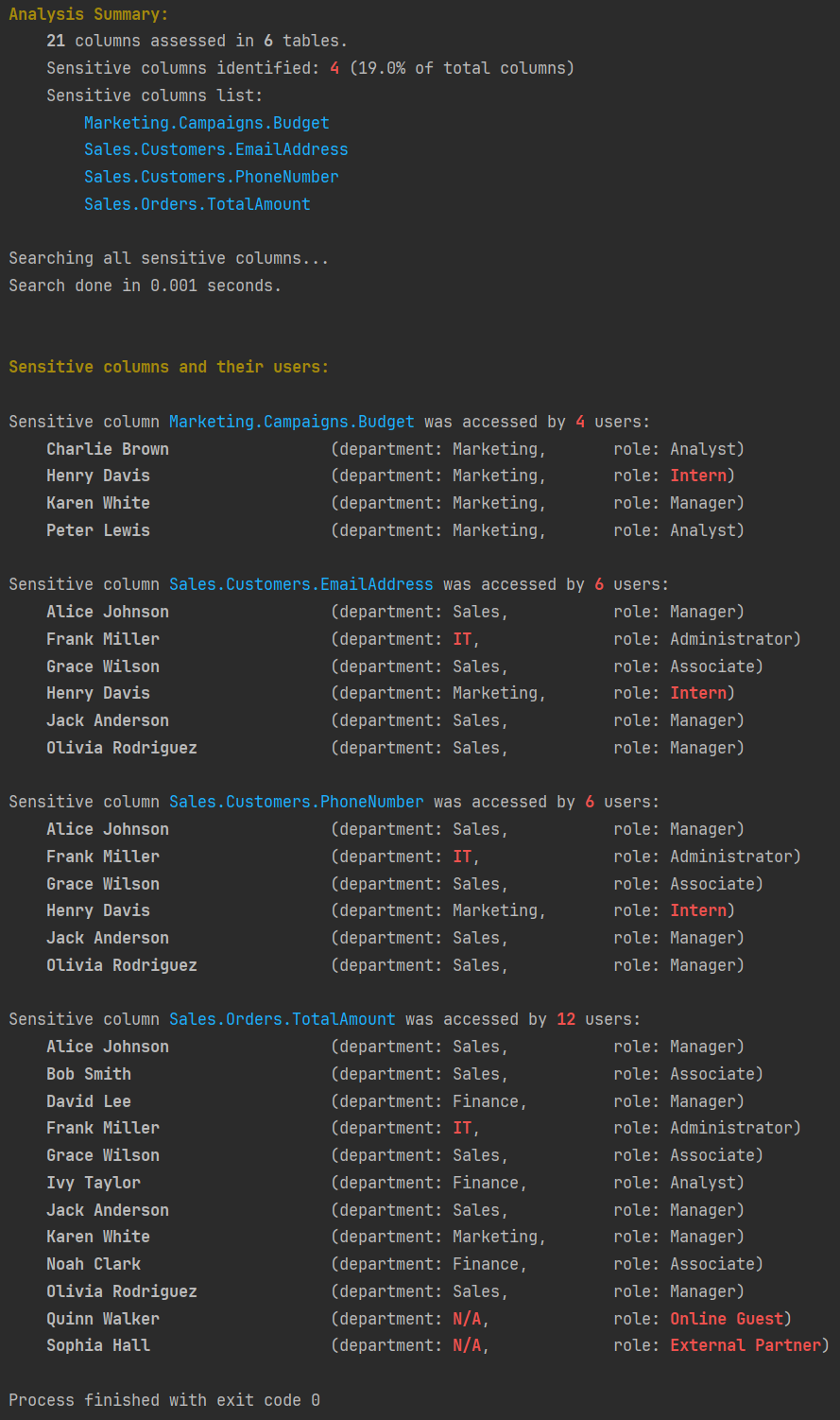
For each sensitive data column, we have a list of users who have accessed it. We have also highlighted potential issues in red. Note that we are capturing search time to measure the efficiency of our algorithm.
Lineage Analysis with Python and NetworkX
Now let us explore the Python code.
We start by reading the data from the three JSON files.
def load_json_from_file(filename):
    with open(filename, "r") as f:
        data = json.load(f)
    return data

database = load_json_from_file('./network-sources/database.json')
reports = load_json_from_file('./network-sources/reports.json')
users = load_json_from_file('./network-sources/users.json')
As the next step, we create a NetworkX graph, which in case of data lineage will be a directed graph - an edge between nodes A and B will either be A-to-B or B-to-A:
G = nx.DiGraph()Now we are ready to build the graph based on JSON content - we will recursively traverse the three JSON files and will build the graph along the way. This is by no means complex but arguably the most tedious part of the code - at each depth of the JSON file we need to create a graph node or an edge:
all_columns = set()
all_sensitive_columns = set()
number_of_tables = 0

for schema in database['database_schemas']:
    G.add_node(schema['name'], type='schema')

    for table in schema['tables']:
        G.add_node(f'{schema['name']}.{table['name']}', type='table')
        G.add_edge(schema['name'], f'{schema['name']}.{table['name']}')
        number_of_tables += 1

        for column in table['columns']:
            G.add_node(f'{schema['name']}.{table['name']}.{column['name']}', type='column', sensitive=column['sensitive'])
            G.add_edge(f'{schema['name']}.{table['name']}', f'{schema['name']}.{table['name']}.{column['name']}')

            all_columns.add(f'{schema['name']}.{table['name']}.{column['name']}')
            if column['sensitive']:
                all_sensitive_columns.add(f'{schema['name']}.{table['name']}.{column['name']}')

for report in reports['reports']:
    G.add_node(report['name'], type='report')

    for report_field in report['report_fields']:
        G.add_node(f'{report['name']}.{report_field['name']}', type='report_field')
        G.add_edge(f'{report['name']}.{report_field['name']}', report['name'])

        # cross-edge:
        for source_column in report_field['source_columns']:
            G.add_edge(source_column, f'{report['name']}.{report_field['name']}')

all_users = {}
for user in users['report_users']:
    G.add_node(user['user_name'], type='user_name', department=user['department'], role=user['role'])
    all_users[user['user_name']] = {"department": (user['department'] if user['department'] else 'N/A'), "role":user['role']}

    # cross-edge:
    for report_viewed in user['reports_viewed']:
        G.add_edge(report_viewed, user['user_name'])
Before we start analysing the data in our graph, let us print out some basic stats - the colour text formatting is done with the colorama library:
total_columns = len(all_columns)
sensitive_count = len(all_sensitive_columns)
sensitive_percentage = (sensitive_count / total_columns) * 100
all_sensitive_columns_sorted_list = sorted(list(all_sensitive_columns))
all_users_sorted_list = sorted(list(all_users))

print(f"{Style.BRIGHT}{Fore.YELLOW}Analysis Summary:{Style.RESET_ALL}")
print(f"\t{Style.BRIGHT}{total_columns}{Style.RESET_ALL} columns assessed in {Style.BRIGHT}{number_of_tables}{Style.RESET_ALL} tables.")
print(f"\tSensitive columns identified: {Style.BRIGHT}{Fore.RED}{sensitive_count}{Style.RESET_ALL} ({sensitive_percentage:.1f}% of total columns)")
print(f"\tSensitive columns list:{Fore.LIGHTBLUE_EX}\n\t\t{"\n\t\t".join(all_sensitive_columns_sorted_list)}{Style.RESET_ALL}")
Now the interesting part - going through all sensitive columns and finding the users that accessed them. Note that we already gathered all sensitive column names into a set when building the graph: all_sensitive_columns.
The easiest way is to iterate through all sensitive columns, for each column iterate through all users and check if the column is connected to the user in our graph.
users_who_viewed_sensitive_column = {}

for sensitive_column in all_sensitive_columns_sorted_list:
    users_who_viewed_sensitive_column[sensitive_column] = list()
    for user in all_users_sorted_list:
        if nx.has_path(G, sensitive_column, user):
            users_who_viewed_sensitive_column[sensitive_column].append(user)
While the above approach will likely be far more efficient than doing the same in a relational database or by traversing the JSON files directly without building a network graph, it is not the best we can do.
To get a rough idea of how long the above search could take with an enterprise-size data set, I executed the above 100,000 times. It was done in 75 seconds.
A more efficient way would be to search only the connected nodes for each sensitive column node:
users_who_viewed_sensitive_column = {}

for sensitive_column in all_sensitive_columns_sorted_list:
    users_who_viewed_sensitive_column[sensitive_column] = list()
    for path in nx.bfs_tree(G, sensitive_column, reverse=False):
        node_data = G.nodes[path]
        if node_data['type'] == 'user_name':
            users_who_viewed_sensitive_column[sensitive_column].append(path)
When executing the above 100,000 times, it is done in 9 seconds - significantly faster. It is likely that this approach will perform well with enterprise-size lineage data.
In the end, we print out the detailed analysis:
def get_user_info(user):

    if all_users[user]["department"] in ["N/A", "IT"]:
        formatted_department = f"{Style.BRIGHT}{Fore.RED}{all_users[user]["department"]}{Style.RESET_ALL}"
    else:
        formatted_department = all_users[user]["department"]

    if all_users[user]["role"] in ["Online Guest", "External Partner", "Intern"]:
        formatted_role = f"{Style.BRIGHT}{Fore.RED}{all_users[user]["role"]}{Style.RESET_ALL}"
    else:
        formatted_role = all_users[user]["role"]

    return f'department: {formatted_department},{" " * (16 - len(all_users[user]["department"]))}role: {formatted_role}'


print(f"\n\n{Style.BRIGHT}{Fore.YELLOW}Sensitive columns and their users:{Style.RESET_ALL}")

for sensitive_column in all_sensitive_columns_sorted_list:
    print(f"\nSensitive column {Fore.LIGHTBLUE_EX}{sensitive_column}{Style.RESET_ALL} was accessed by {Style.BRIGHT}{Fore.RED}{len(users_who_viewed_sensitive_column[sensitive_column])}{Style.RESET_ALL} users:")
    for user in users_who_viewed_sensitive_column[sensitive_column]:
        print(f"\t{Style.BRIGHT}{user}{Style.RESET_ALL}{" " * (30 - len(user))}({get_user_info(user)})")
Conclusion
Python, with its versatile NetworkX library, offers an efficient and accessible entry point for network graph analysis, providing capabilities such as shortest path finding, connectivity testing, and community detection. While more powerful libraries exist, NetworkX excels in ease of use and rapid prototyping, making it an ideal choice for those starting their journey in graph analysis with Python. With proper implementation, NetworkX can also deliver impressive performance.